Miscellaneous operators
This page covers FuseQL operators and reference material that do not fit a larger category: time-shifted comparison, forecasting, and reserved field names.
compare timeshift
Adds one or more columns containing time-shifted historical values alongside the current aggregated data. Use compare timeshift to perform day-over-day, week-over-week, or custom-period comparisons in a single query — each shifted column contains the metric value from the specified duration ago.
|
|
Syntax
| compare timeshift <duration>
| compare timeshift <duration> <count>
| compare timeshift <duration> as <alias>
| compare timeshift <duration> as <alias>, timeshift <duration2> as <alias2>Parameters
| Parameter | Required | Description |
|---|---|---|
|
Required |
How far back to shift. Supported units: |
|
Optional |
Number of shifted periods to generate. Creates |
|
Optional |
Custom name for the comparison column. Without an alias, columns are named |
Multiple timeshifts |
Optional |
Specify additional |
Example
Compare hourly nginx request counts with both yesterday and last week.
source="nginx"
| timeslice 1h
| count by (_timeslice)
| compare timeshift 1d as yesterday, timeshift 1w as last_week| _timeslice | _count | count_yesterday | count_last_week |
|---|---|---|---|
2026-06-27 18:00:00 UTC |
650,712 |
598,240 |
612,450 |
2026-06-27 19:00:00 UTC |
474,040 |
441,800 |
488,920 |
|
Rows return |
compose
Converts query results into a FuseQL filter expression (a boolean OR of field=value conditions). compose is primarily used as the final stage of a subquery, but can also be run standalone to preview the generated filter. Use it to dynamically build filters from aggregated data — for example, generating a filter from the top error-producing hosts discovered in one query and applying it to another.
Parameters
| Parameter | Required | Description |
|---|---|---|
|
Required |
One or more field names. Multiple fields create AND conditions within each row; rows are combined with OR. |
|
Optional |
Limits the number of result rows used in filter generation. Default: |
|
Optional |
Generates keyword grep searches ( |
Example
Generate a filter from the level and org_id combinations found in query-service logs, then use it to filter another source.
source="query-service"
| count by level, org_id
| compose level, org_id| _filter |
|---|
level="error" and org_id="pisco-shared") or (level="info" and org_id="pisco-shared" |
|
none Run |
Linear Forecast
Forecasts future metric values by fitting a linear regression model to historical time-series data. Use Linear Forecast when your data shows a consistent upward or downward trend without strong seasonal patterns — for example, predicting steady traffic growth or a declining error rate.
Linear forecasting is built on the Linear Regression. It extrapolates the trend line forward for a specified duration.
Parameters
| Parameter | Required | Description |
|---|---|---|
|
Required |
The aggregated numeric field to forecast. |
|
Required |
The time bucket size matching the upstream |
|
Required |
Selects the linear regression model. |
|
Required |
How far forward to project. Expressed in seconds (e.g., |
Example


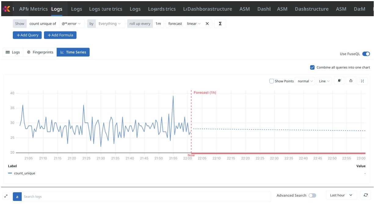
|
Linear forecasting works best for data with a clear monotonic trend. For data with hourly or daily cyclical patterns, use Seasonal Forecast instead. The |
Reserved fields
FuseQL provides a set of reserved field names that map to the core columns shown in the Log Search results view. Use these fields to filter, extract, or alias the primary log attributes without parsing them from the raw log line.
Field reference
| Field | Maps to | Description |
|---|---|---|
|
Message column |
The full raw log line text. Regex matching against |
|
Level column |
The log severity level (e.g., |
|
Source column |
The log source identifier (equivalent to the |
Example
Filter logs by message pattern, level, and source simultaneously using reserved fields.
__kf_msg =~ "ERROR.*connection.*timeout"
__kf_level = "ERROR"
__kf_source = "nginx"Alias example
Reorder the default log columns by aliasing reserved fields. Using aliases disables the default column display and shows only the aliased versions in the result.
* | __kf_msg as LogMessage | __kf_level as LogLevel | __kf_source as LogSource|
Reserved fields are available in all FuseQL contexts — filter expressions, |
Seasonal Forecast
Forecasts future metric values from time-series data that contains recurring seasonal patterns — hourly, daily, or weekly cycles — in addition to overall trends. Use Seasonal Forecast when your data shows predictable periodic behavior, such as traffic spikes every morning or error rate increases every evening.
Seasonal forecasting is built on Prophet, which handles seasonality, trend, and holiday effects simultaneously.
Syntax
| predict (<field>) by <bucket_size>, model=seasonal, seasonality=<period>, forecast=<duration>Parameters
| Parameter | Required | Description |
|---|---|---|
|
Required |
The aggregated numeric field to forecast. |
|
Required |
The time bucket size matching the upstream |
|
Required |
Selects the seasonal (Prophet) model. |
|
Required |
The dominant seasonal period. Supported values: |
|
Required |
How far forward to project. Expressed in seconds (e.g., |
Example
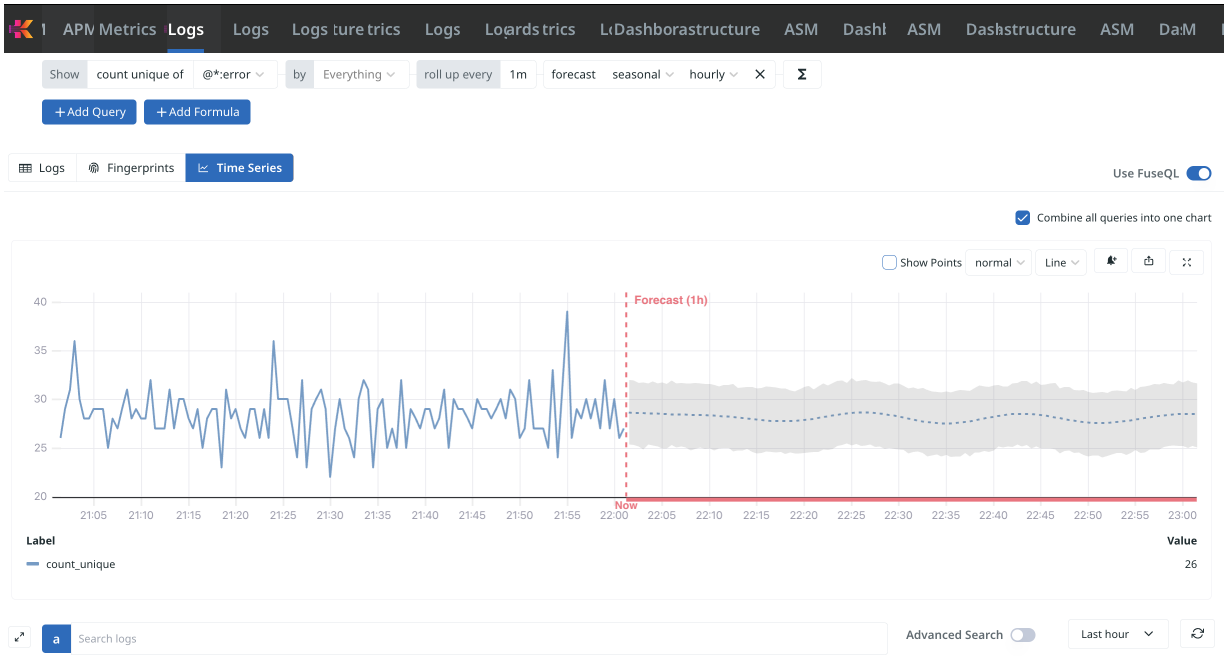
|
Use |
subquery
Executes a nested inner query, converts its results into a filter expression using compose, and applies that filter to the outer query. Use subquery to correlate data across sources without manual copy-paste — for example, finding all logs from hosts that also appear in a separate error log source.
|
The |
Syntax
[subquery: <inner_query> | compose <fields> [maxresults=<N>] [keywords]]The subquery block can appear in three positions:
[subquery: <inner_query> | compose <fields>] | <outer_query>

<outer_query> | where [subquery: <inner_query> | compose <fields>]

<outer_query> | if([subquery: <inner_query> | compose <fields>], <true_value>, <false_value>) as <field>Parameters
| Parameter | Required | Description |
|---|---|---|
|
Required |
Any valid FuseQL query. Its results are passed to |
|
Required |
Converts the inner query’s result rows into a boolean filter expression. |
|
Optional |
Limits how many result rows |
|
Optional |
Generates keyword grep searches instead of field equality filters. Not supported with |
Example
Filter logs from org_id="pisco-shared" to only those originating from hosts that also appear in query-service logs.
org_id="pisco-shared"
and [subquery: source="query-service" | count by host | compose host]
| timeslice 20s
| count by _timesliceThe inner query produces:
| host | _count |
|---|---|
server-1 |
250 |
server-2 |
180 |
compose host converts this to host="server-1") or (host="server-2", making the full query equivalent to:
org_id="pisco-shared"
and ((host="server-1") or (host="server-2"))
| timeslice 20s | count by _timeslice|
Always test the outer query independently before adding the inner subquery. Subqueries within |
topk
The topk operator keeps the highest-ranked rows of an aggregation result. Use it to answer questions like "the top 5 hosts by error count" or "the top 3 endpoints by latency per service".
topk runs after an aggregation. It sorts the aggregated rows in descending order by a ranking field, keeps at most k rows, and adds a rank column starting at 1. With a by clause, topk ranks within each group independently and returns the top _k rows for every group.
Syntax
| topk(<k>, <ranking_field>)
| topk(<k>, <ranking_field>) by <field1>, <field2>, ...<k>-
Positive integer. The maximum number of rows to keep. Must be
>= 1. If fewer rows exist thank, all rows are returned. <ranking_field>-
The field used to rank rows in descending order. This is typically an aggregation output column such as
_count, or an aliased aggregation likeerrorsfromcount as errors. by <field1>, <field2>, …-
Optional grouping fields. When present,
topkpartitions input rows by the listed fields and returns the top k rows within each group. Group order in the output follows the order in which each group is first seen in the input.
Output
topk appends a _rank column to the schema. _rank is 1 for the highest-ranked row in each result set (or per group), 2 for the next, and so on. Within a by group, _rank restarts at 1.
Rows are ordered:
-
Globally (no
byclause): descending by<ranking_field>. -
Per group (
byclause): groups appear in input order; within each group, rows are descending by<ranking_field>.
Behavior
-
topkmust appear after an aggregation operator such ascount,sum,avg, orpercentiles. Usingtopkbefore an aggregation returns an error. -
Comparison is numeric when both values being compared are numeric (including mixed
intandfloatvalues); otherwise the values are compared as strings. -
Missing or
nullranking values sort to the end, so rows with no value never appear in the top results unlesskexceeds the number of non-null rows. -
A
topkwith a value of<k>that is larger than the input set is not an error —topkreturns all input rows.
Example: Top N across all results
Return the 5 sources producing the most logs:
* | count by source | topk(5, _count)The result has at most 5 rows ranked by _count descending, with _rank values 1 through 5.