Holt Winters
The Holt-Winters function produces a smoothed value for time series based on the range in the time series, accounting for seasonal adjustments. Implements the Holt-Winters method of exponentially-weighted averages as smoothing factors.
Parameters
- sf
-
The smoothing factor, where lower values weigh towards the importance of older data.
Valid values for this scalar parameter must be between 0 and 1.
- tf
-
The trend factor, where higher values weigh in favor of trends in the time series.
Valid values for this scalar parameter must be between 0 and 1.
How it works
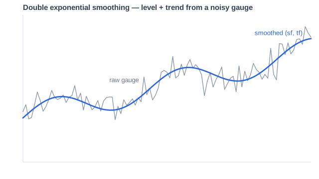
Double exponential smoothing maintains two running estimates per series — the current level and the current trend — and updates both exponentially with every sample: sf controls how strongly new samples move the level, tf how strongly recent movement updates the trend. The output is the smoothed level, producing a stable signal from a noisy gauge.
In Dashboards
The holt_winters function is not supported in Kloudfuse PromQL.
|
Double exponential smoothing is available under its current Prometheus name, double_exponential_smoothing, which takes the same smoothing factor (sf) and trend factor (tf) parameters. See double_exponential_smoothing in the PromQL documentation.
Limitations
-
No seasonality. The available form,
double_exponential_smoothing, models level and trend only — it does not learn repeating patterns. For seasonal data, use SARIMA, Prophet, or Seasonal Decompose instead. -
Fixed factors, no fitting.
sfandtfare constants you choose per query; nothing tunes them to the data. Factors that suit one metric can over-smooth or under-smooth another. -
Lags sudden changes. Exponential smoothing responds gradually by design — a step change in the metric appears in the output only after several samples, and lower
sfvalues increase that lag. -
Smoothing only, no bands. The function returns one smoothed series; it does not produce upper and lower bounds, so it is not an anomaly detector by itself.
-
Additive assumptions. The method assumes trend and noise combine additively; multiplicative behavior (variance that grows with the level) is smoothed poorly.
-
Use only with Gauge metric types — smoothing a raw counter smooths its monotonic growth, not its rate.
Background
Holt-Winters was initially developed in 1957 by Charles Holt (Holt), and later extended by his student Peter Winters in 1960 (Winters) to introduce a trend component to represent seasonality. The method has performed well in many situations, but it was originally developed for a specific type of data — trend-seasonal. The original method also implies that noise has an additive form, while the seasonality is multiplicative.
Many advancements in forecast modeling took place in the intervening years, including the development of the ETS framework in 2008 (Hyndman et al.), which covers 30 possible models for time series with different types of error, trend, and seasonal components. The Holt-Winters Seasonal method aligns with only one of the models in the framework.
For an in-depth discussion, see Why you should not use Holt-Winters method by Ivan Svetunkov.