Seasonal Decompose
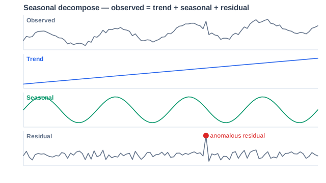
Seasonal Decompose splits each time series into trend, seasonal, and residual components, and flags anomalies where the residual departs from its expected band.
Parameters
- period
-
Number of data points per season — 1440 at 1-minute resolution for daily seasonality.
- model
-
0 = additive decomposition, 1 = multiplicative.
- window
-
Number of milliseconds in the smoothing window — 1,800,000 ms for a 30-minute window.
- bound
-
Width of the band in standard deviations: 1, 2, or 3.
- band
-
Which band series to return: 4 = lower band, 5 = upper band, 6 = both.
How it works
To calculate the prediction bounds, refer to the STL Decomposition.ipynb notebook that investigates the option of adding the mean and the standard deviations of the residuals into the trend and seasonal components.
lower = avg_over_time(
  (mean_over_time(Residuals[5m:])
  -$Bound*stddev_over_time(Residuals[5m:]))[5m:])
  + Trend
+ Seasonal Componentupper = avg_over_time(
(mean_over_time(Residuals[5m:])
+$Bound*stddev_over_time(Residuals[5m:]))[5m:])
+ Trend
+ Seasonal ComponentIn Dashboards
To use the seasonal_decompose operator in a dashboard, apply the following function:
seasonal_decompose( \
  ${promql}, \ (1)
  ${period}, \ (2)
  ${model}, \ (3)
  ${window}, \ (4)
  ${bound}, \ (5)
  ${band} \ (6)
)| 1 | ${promql}: PromQL query to evaluate |
| 2 | ${period}: Number of data points per season — 1440 at 1-minute resolution for daily seasonality |
| 3 | ${model}: 0 = additive decomposition, 1 = multiplicative |
| 4 | ${window}: Number of milliseconds in the window (1,800,000 ms for a 30-minute window) |
| 5 | ${bound}: Number of standard deviations (stdv): 1, 2, or 3 |
| 6 | ${band}: 4 = lower band, 5 = upper band, 6 = both upper and lower bands |
For the operator reference — syntax, parameters, and a validated example — see seasonal_decompose in the PromQL documentation.
Limitations
-
If the evaluated metrics do not exhibit true seasonality, Seasonal Decompose may create incorrect (invalid) alerts, or mask valid alerting conditions.
-
The algorithm requires at least 2 ×
periodof history, which the service fetches beyond the visible chart range. If retention or the metric’s age cannot supply it, the series produces no result. -
The model is computed per input series; reduce series count with an aggregation before applying.
-
periodmust match the data’s true season length in data points at the query resolution — a mismatched period produces bands that look plausible but are meaningless.
Next steps
For an in-depth discussion of the Seasonal Decomposition approach, see these resources:
-
Documentation for statsmodels.tsa.seasonal.seasonal_decompose
-
Decomposition of time series in Wikipedia
-
Time-Series-Analysis/STL Decomposition.ipynb GitHub repository