Algorithmic operators
FuseQL provides algorithmic operators for detecting unexpected behavior in time-series data. These operators apply statistical models to identify anomalies and highlight outlier series.
Anomaly detection
Anomaly detection is a powerful monitoring feature that uses algorithmic analysis to automatically identify unexpected behavior in metric data. Traditional threshold-based alerting often fails to account for trends, seasonality, or complex fluctuations in metrics.
Anomaly detection algorithms overcome this limitation by analyzing historical patterns to establish dynamic boundaries (bounds), making it possible to detect deviations from normal behavior even as the data changes over time.
In practice, anomaly functions overlay a band on the metric, showing the expected behavior of a series based on past values.
Kloudfuse provides four anomaly detection models.
- basic
-
Implements the Rolling quantile algorithm.
- agile
-
Uses the SARIMA model.
- robust
-
The robust anomaly detection algorithm uses a Seasonal Decompose.
- agile-robust
-
Applies the Prophet model.
Basic anomaly detection
Implements the Rolling quantile algorithm.
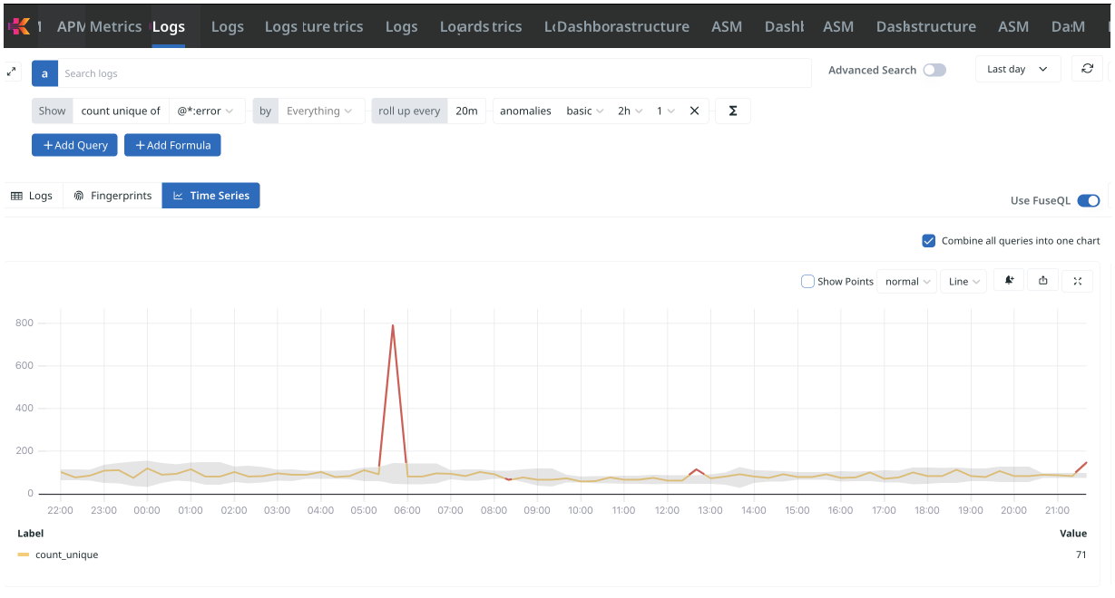
This algorithm calculates a predicted range using the 25th and 75th quantiles and the interquartile range (IQR) within a rolling window. This range determines the expected normal behavior; deviations outside this range are anomalies.
Basic anomaly detection is ideal for monitoring metrics with frequent, non-seasonal fluctuations, where rapid response to changes is essential. Use it to detect unexpected spikes or drops without needing to account for cyclic patterns or trends.
Parameters
- window
-
Defines the size of the rolling window for quantile computation. A larger window smooths the data, but reduces sensitivity to sudden changes.
- bounds
-
Set the sensitivity of anomaly detection. Narrower bounds make the algorithm more sensitive to deviations, while wider bounds classify more data as normal.
-
Bounds:1 (Narrow) Offers high sensitivity by setting a tighter range around predicted values, detecting even minor deviations. This band is useful when you need to capture subtle changes in log volume that might indicate early signs of issues.
-
Bound 2 (Moderate): Provides a moderate range, making the algorithm less sensitive to minor fluctuations and ideal for monitoring with fewer false positives.
-
Bound 3 (Wide): Defines the widest range, capturing only significant deviations. This setting is suitable for metrics where only large, impactful anomalies are of interest, reducing alert noise for minor variations.
-
Example


The time series graph displays a unique count of errors over a period. The gray band represents the expected range based on recent data, while red markers indicate anomalies — data points outside the predicted range. Here, a sudden increase in errors during peak hours is flagged as an anomaly, helping with quick detection and investigation.
Agile anomaly detection
Parameters
- Seasonality
-
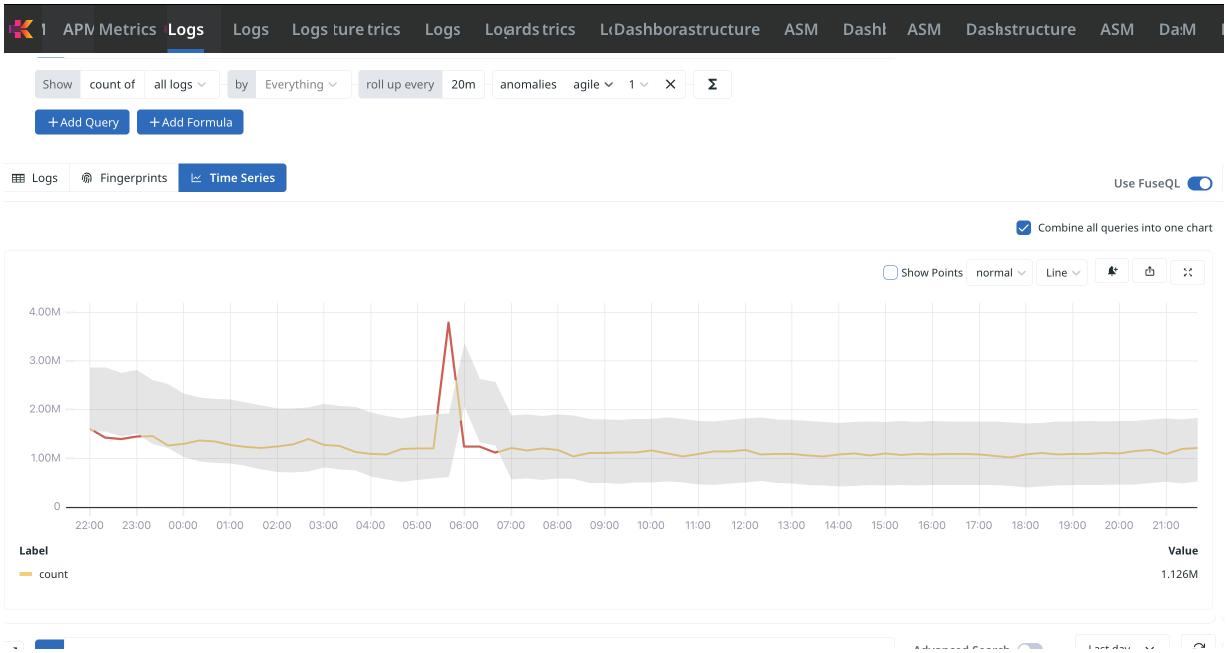
The algorithm auto-detects the seasonality, either hourly or daily:
-
Hourly: Logs metrics that display hourly cyclic behavior. If your log data typically fluctuates each hour based on user activity or background processes, hourly seasonality enables the SARIMA model to capture these hourly patterns accurately.
-
Daily: Captures daily seasonality, suitable for log metrics with a daily recurring pattern. If log entries spike every evening due to daily system maintenance tasks, the Daily option allows the model to recognize these daily trends.
-
- bounds
-
Set the sensitivity of anomaly detection. Narrower bounds make the algorithm more sensitive to deviations, while wider bounds classify more data as normal.
-
Bounds:1 (Narrow) Offers high sensitivity by setting a tighter range around predicted values, detecting even minor deviations. This band is useful when you need to capture subtle changes in log volume that might indicate early signs of issues.
-
Bound 2 (Moderate): Provides a moderate range, making the algorithm less sensitive to minor fluctuations and ideal for monitoring with fewer false positives.
-
Bound 3 (Wide): Defines the widest range, capturing only significant deviations. This setting is suitable for metrics where only large, impactful anomalies are of interest, reducing alert noise for minor variations.
-

Robust anomaly detection
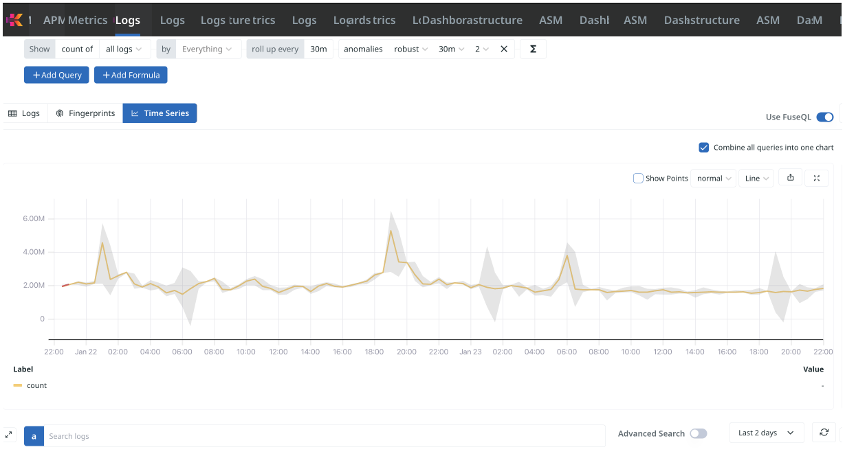
The Robust anomaly detection algorithm uses a Seasonal Decompose technique to identify anomalies in time series data. Seasonal decomposition separates the data into its seasonal, trend, and residual components, and enables more accurate anomaly detection in metrics with strong seasonal patterns.
Parameters
- Rolling Window size
-
Calculate the standard deviation (stddev) for anomaly detection, and to set the bounds for the expected values.
A larger window has a smoother, more stable standard deviation calculation. However, it is less responsive to sudden, short-term spikes or drops.
A smaller window size is more responsive to recent data points, and enables a quicker reaction to changes. However, it results in more
noise. - bounds
-
Set the sensitivity of anomaly detection. Narrower bounds make the algorithm more sensitive to deviations, while wider bounds classify more data as normal.
-
Bounds:1 (Narrow) Offers high sensitivity by setting a tighter range around predicted values, detecting even minor deviations. This band is useful when you need to capture subtle changes in log volume that might indicate early signs of issues.
-
Bound 2 (Moderate): Provides a moderate range, making the algorithm less sensitive to minor fluctuations and ideal for monitoring with fewer false positives.
-
Bound 3 (Wide): Defines the widest range, capturing only significant deviations. This setting is suitable for metrics where only large, impactful anomalies are of interest, reducing alert noise for minor variations.
-
Agile-Robust anomaly detection
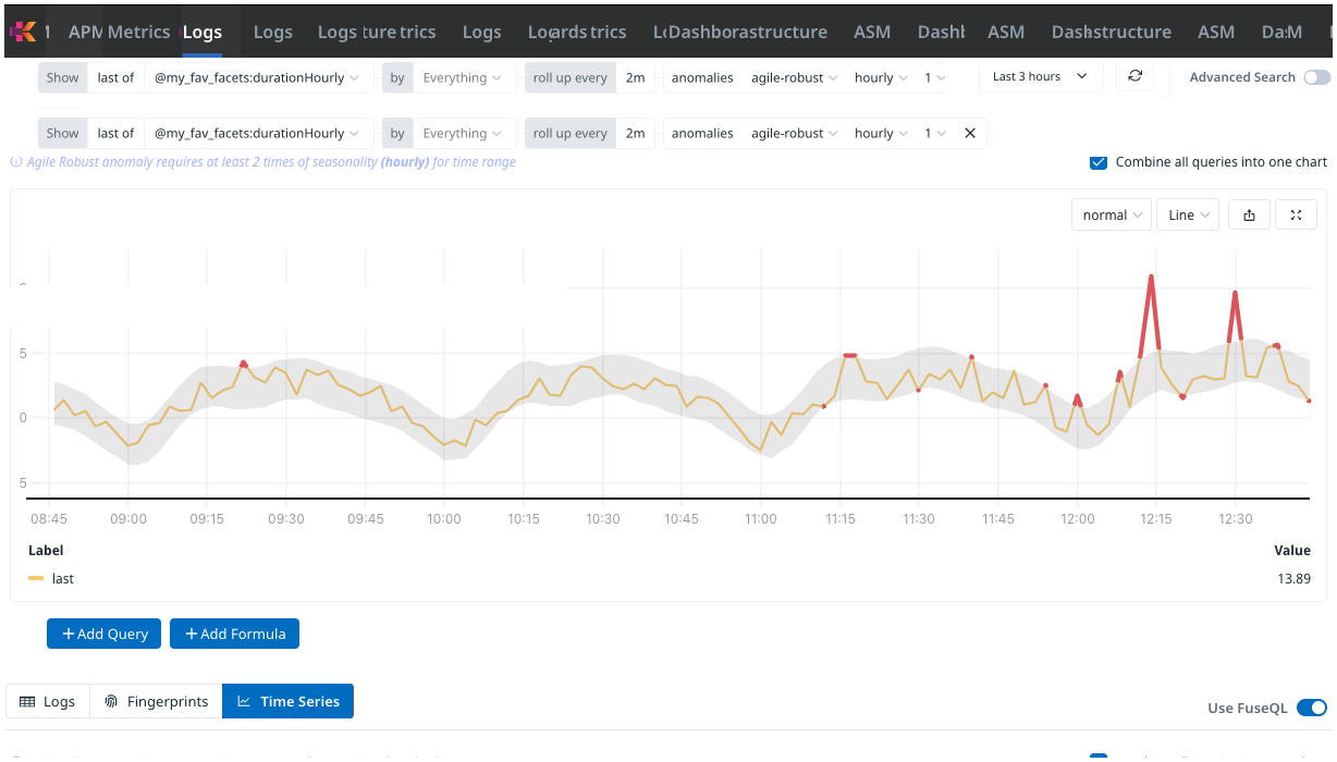
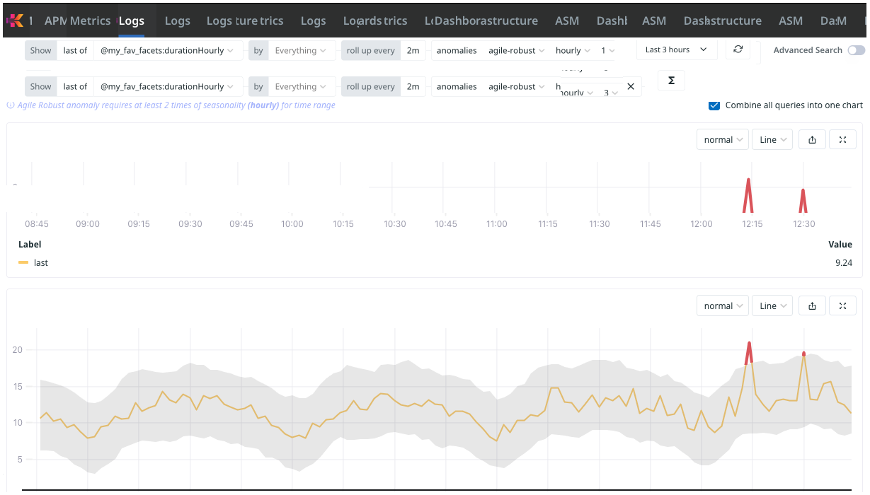
Applies the Prophet model to detect anomalies in log metrics with recurring patterns and occasional level shifts. This approach identifies irregularities in logs that exhibit seasonal behaviors, such as error spikes, request rates, or event frequencies, which follow daily or hourly patterns.
Parameters
- Seasonality
-
The algorithm auto-detects the seasonality, either hourly or daily:
-
Hourly: Logs metrics that display hourly cyclic behavior. If your error logs tend to spike each hour due to automated checks or periodic background processes, the Hourly option enables the Prophet algorithm to model these regular occurrences and detect deviations that fall outside the norm.
-
Daily: Captures daily seasonality, suitable for log metrics with a daily recurring pattern. You may observe an expectant daily surge in user login errors each morning when users start their workday. With Daily seasonality, the algorithm anticipates these recurring daily trends, flagging only unusual changes outside the expected pattern.
-
Outlier detection
Kloudfuse uses the Outliers function to highlight outlier time series.
DBSCAN
Kloudfuse provides the DBSCAN implementation of outlier detection.
Visualization
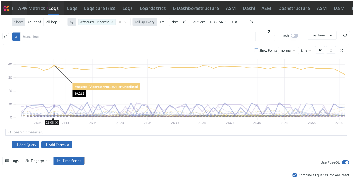
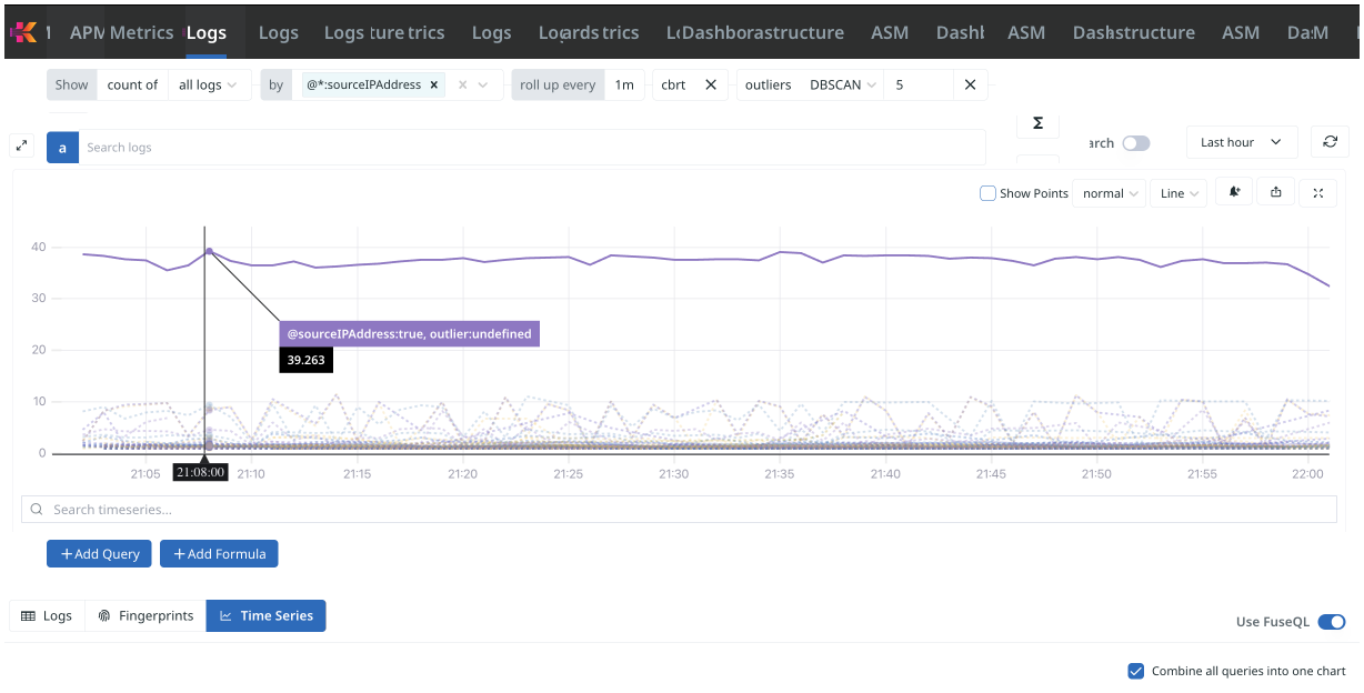
The chart displays the results of DBSCAN outlier detection, applied to the selected log metric over time.
-
Solid Lines represent data series flagged as outliers. These indicate instances where the data behavior deviates significantly from the norm, based on the defined tolerance.
-
Dotted Lines represent data series identified as non-outliers, because they exhibit expected behavior relative to their peers.
Search
Use the Search time series option (below the graph) to select and plot the relevant information. For example, you can search for outlier:true to paint only the series that have outlier data.
As with all linear plots, you can select and deselect lines using the Label legend.
Examples
Tolerance of 0.8
The choice of tolerance value in this example makes the detection process highly sensitive to deviations. The algorithm detects and reports even small deviations from the normal pattern.